NLP : Text classification of BBC news dataset

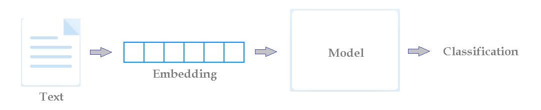
This project is about text classification ie: given a text, we would want to predict its class (tech, business, sport, entertainment or politics).

My github repository for this project is here

We will be using “BBC-news” dataset ( available in Kaggle ) to do following steps:

• Pre-process the dataset
• Build 3 types of model to classify sentences into 5 categories ( tech, business, sport, entertainment, politics )
• Compare models performance
• Visualisation of the word embedding in 2D using PCA
• Visualisation of the word embedding in 3D using T-SNE

Downloading Dataset

!wget --no-check-certificate \
    https://storage.googleapis.com/laurencemoroney-blog.appspot.com/bbc-text.csv \
    -O /tmp/bbc-text.csv

I’ll start by defining some parameters values for the pre-processing step:

vocab_size = 1000
embedding_dim = 16
max_length = 120
trunc_type='post'
padding_type='post'
oov_tok = "<OOV>"
training_portion = .8

Below is the list of the stopwords that dont influence on the meaning of the sentences.

stopwords = [ "a", "about", "above", "after", "again", "against", "all", "am", "an", "and", "any", "are", "as", "at", "be", "because", "been", "before", "being", "below", "between", "both", "but", "by", "could", "did", "do", "does", "doing", "down", "during", "each", "few", "for", "from", "further", "had", "has", "have", "having", "he", "he'd", "he'll", "he's", "her", "here", "here's", "hers", "herself", "him", "himself", "his", "how", "how's", "i", "i'd", "i'll", "i'm", "i've", "if", "in", "into", "is", "it", "it's", "its", "itself", "let's", "me", "more", "most", "my", "myself", "nor", "of", "on", "once", "only", "or", "other", "ought", "our", "ours", "ourselves", "out", "over", "own", "same", "she", "she'd", "she'll", "she's", "should", "so", "some", "such", "than", "that", "that's", "the", "their", "theirs", "them", "themselves", "then", "there", "there's", "these", "they", "they'd", "they'll", "they're", "they've", "this", "those", "through", "to", "too", "under", "until", "up", "very", "was", "we", "we'd", "we'll", "we're", "we've", "were", "what", "what's", "when", "when's", "where", "where's", "which", "while", "who", "who's", "whom", "why", "why's", "with", "would", "you", "you'd", "you'll", "you're", "you've", "your", "yours", "yourself", "yourselves" ]

Reading the dataset and removing the stopwords

After this lines of codes, sentences and labels is 2 lists that contain 2225 values each.

sentences = []
labels = []
with open("/tmp/bbc-text.csv", 'r') as csvfile:
    reader = csv.reader(csvfile, delimiter=',')
    next(reader)
    for row in reader:
        labels.append(row[0])
        sentence = row[1]
        for word in stopwords:
            token = " " + word + " "
            sentence = sentence.replace(token, " ")
        sentences.append(sentence)

Pre-processing of data

We will start by splitting it into training and validation parts using the ratio “training_portion = 0.8”

train_size = int(len(sentences) * training_portion)
#training
train_sentences = sentences[:train_size]
train_labels = labels[:train_size]
#validation
validation_sentences = sentences[train_size:]
validation_labels = labels[train_size:]

The code below is for tokenization and padding of each sentences into a tokenized array with length 120.

from tensorflow.keras.preprocessing.text import Tokenizer
from tensorflow.keras.preprocessing.sequence import pad_sequences

tokenizer = Tokenizer(num_words = vocab_size, oov_token=oov_tok)
tokenizer.fit_on_texts(train_sentences)
word_index = tokenizer.word_index
#training
train_sequences = tokenizer.texts_to_sequences(train_sentences)
train_padded = pad_sequences(train_sequences, padding=padding_type, maxlen=max_length)
#validation
validation_sequences = tokenizer.texts_to_sequences(validation_sentences)
validation_padded = pad_sequences(validation_sequences, padding=padding_type, maxlen=max_length)

We will also tokenize labels into 6 classes ( tech, business, sport, entertainment, politics, OOV ), the additional class is for out of vocabulary.

label_tokenizer = Tokenizer()
label_tokenizer.fit_on_texts(labels)
#training
training_label_seq = np.array(label_tokenizer.texts_to_sequences(train_labels))
#validation
validation_label_seq = np.array(label_tokenizer.texts_to_sequences(validation_labels))

Building models for sentence classification

We wil start by the most simple one with 24 Denses layers

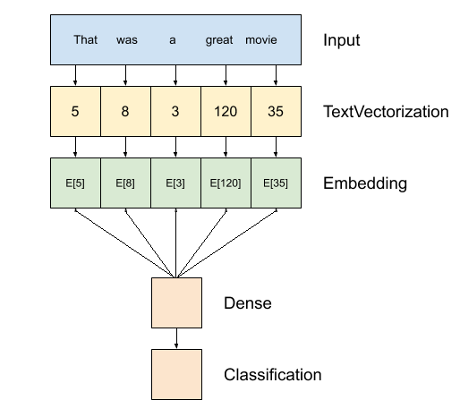
model_64_dense = tf.keras.Sequential([
    tf.keras.layers.Embedding(vocab_size, embedding_dim, input_length=max_length),
    tf.keras.layers.GlobalAveragePooling1D(),
    tf.keras.layers.Dense(24, activation='relu'),
    tf.keras.layers.Dense(6, activation='softmax')
])
model_64_dense.compile(loss='sparse_categorical_crossentropy',optimizer='adam',metrics=['accuracy'])
history = model_64_dense.fit(train_padded, training_label_seq, epochs=num_epochs, validation_data=(validation_padded, validation_label_seq), verbose=2)

Next, is an LSTM of 32 units

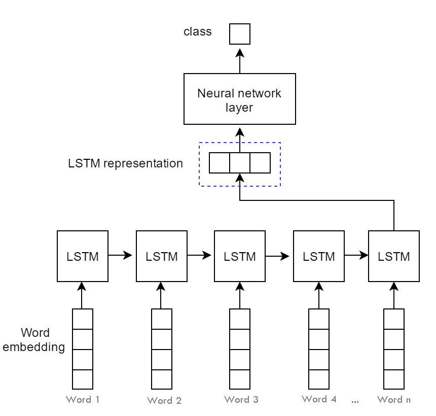
model_32_LSTM = tf.keras.Sequential([
    tf.keras.layers.Embedding(vocab_size, embedding_dim, input_length=max_length),
    tf.keras.layers.LSTM(32),
    #tf.keras.layers.Dense(24, activation='relu'),
    tf.keras.layers.Dense(6, activation='softmax')
])
model_32_LSTM.compile(loss='sparse_categorical_crossentropy',optimizer='adam',metrics=['accuracy'])
history2 = model_32_LSTM.fit(train_padded, training_label_seq, epochs=60, validation_data=(validation_padded, validation_label_seq), verbose=2)

The last one has Con1D in addition to LSTM:

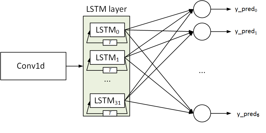
model_lstm_conv1d = tf.keras.Sequential([
    tf.keras.layers.Embedding(vocab_size, embedding_dim, input_length=max_length),
    tf.keras.layers.Dropout(0.2),
    tf.keras.layers.Conv1D(64, 5, activation='relu'),
    tf.keras.layers.MaxPooling1D(pool_size=4),
    tf.keras.layers.LSTM(64),
    tf.keras.layers.Dense(6, activation='softmax')
])
model_lstm_conv1d.compile(loss='sparse_categorical_crossentropy',optimizer='adam',metrics=['accuracy'])
history3 = model_lstm_conv1d.fit(train_padded, training_label_seq, epochs=num_epochs, validation_data=(validation_padded, validation_label_seq), verbose=2)

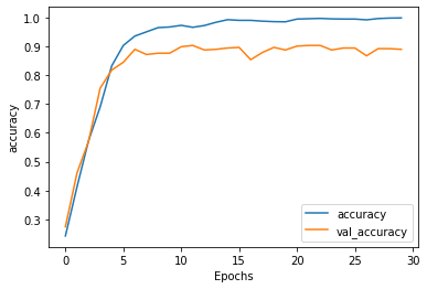
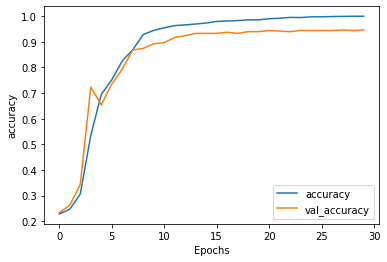
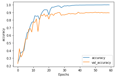
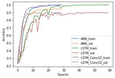
Comparison of performance between the 3 models

plt.plot(history.history['accuracy'])
plt.plot(history.history['val_'+'accuracy'],'--')
plt.plot(history2.history['accuracy'])
plt.plot(history2.history['val_'+'accuracy'],'--')
plt.plot(history3.history['accuracy'])
plt.plot(history3.history['val_'+'accuracy'],'--')
plt.xlabel("Epochs")
plt.ylabel('accuracy')
plt.legend(['ANN_train','ANN_val','LSTM_train','LSTM_val','LSTM_Conv1D_train','LSTM_Conv1D_val'])
plt.show()

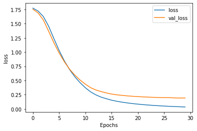
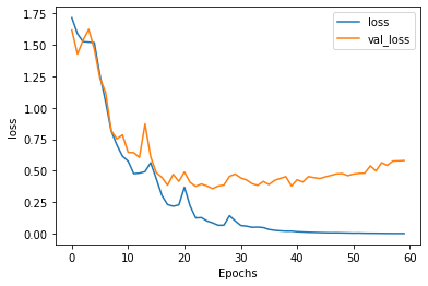
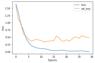
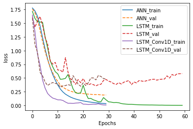
plt.plot(history.history['loss'])
plt.plot(history.history['val_'+'loss'],'--')
plt.plot(history2.history['loss'])
plt.plot(history2.history['val_'+'loss'],'--')
plt.plot(history3.history['loss'])
plt.plot(history3.history['val_'+'loss'],'--')
plt.xlabel("Epochs")
plt.ylabel('loss')
plt.legend(['ANN_train','ANN_val','LSTM_train','LSTM_val','LSTM_Conv1D_train','LSTM_Conv1D_val'])
plt.show()

Extracting embedding layer’s weights from each model

The weights matrix has a shape of (1000, 16) with 1000 = vocab_size and 16=emb_dim

x=model_64_dense.layers[0]
weight1=x.get_weights()[0]
y=model_32_LSTM.layers[0]
weight2=y.get_weights()[0]
z=model_lstm_conv1d.layers[0]
weight3=z.get_weights()[0]

Here, we define a function that decodes a token into a word

reverse_word_index = dict([(value, key) for (key, value) in word_index.items()])

def decode_sentence(text):
    return ' '.join([reverse_word_index.get(i, '?') for i in text])

(Optional): the code below is for the euclidian distance and cosine similarity

from numpy import dot
from numpy.linalg import norm

def cos_sim(a,b):
  return dot(a, b)/(norm(a)*norm(b))

def euc_dist(a,b):
  return np.linalg.norm(a-b)

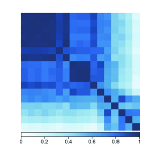
Correlation matrix, Eigen Values/Vectors and PCA

import pandas as pd
df=pd.DataFrame(weight1)
X_corr=df.corr()

values,vectors=np.linalg.eig(X_corr)
eigv_s=(-values).argsort()
vectors=vectors[:,eigv_s]
new_vectors=vectors[:,:2]
new_X=np.dot(weight1,new_vectors)

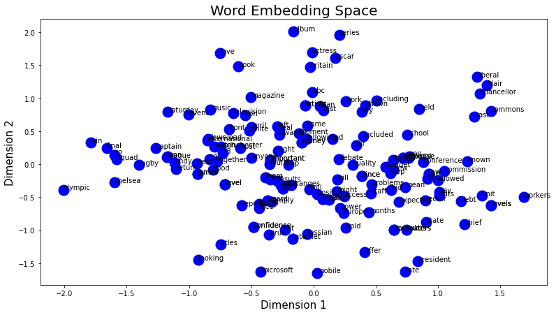
Here, we reduced the embedding dimension from 16 to 2 ie: we’ve chosen the 2 eigen vectors (x1,x2) that have the highest eigen values then we did a dot product between the embedding matrix of shape (1000,16) and the new vector of shape (16,2).

import matplotlib.pyplot as plt
vocab_word=list(word_index.keys())
vocab_word=vocab_word[:1000]
random_vocab=np.random.choice(vocab_word,150)
random_index=list(word_index[i] for i in random_vocab)
sampled_X=new_X[random_index,:]
plt.figure(figsize=(13,7))
plt.scatter(sampled_X[:,0],sampled_X[:,1],linewidths=10,color='blue')
plt.xlabel("Dimension 1",size=15)
plt.ylabel("Dimension 2",size=15)
plt.title("Word Embedding Space",size=20)
vocab=len(random_vocab)
for i in range(vocab):
  word=random_vocab[i]
  plt.annotate(word,xy=(sampled_X[i,0],sampled_X[i,1]))

Below is the visualisation of the word embedding of the “BBC news” dataset in 2D.

Word embedding in 3D using T-SNE

Here is the T-SNE visualisation of the word embedding in 3D. It was done using “Embedding Projector” with 5035 iterations and 25 perplexity.

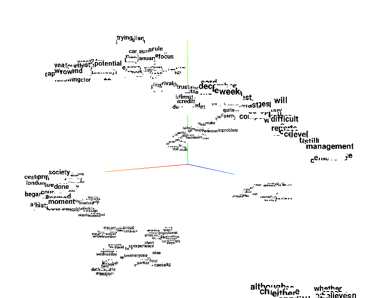
We can see that the embedding is divided into 6 groups of words. In fact, each one contains words that are specific to each class.

Conclusion

This project was about classifying text using “BBC news” dataset, comparing between different models performances and visualizing word embedding using PCA and T-SNE.